NBA Stat Predictor
Project Overview
Built a model to predict NBA Player Season Stats that outperformed ESPN’s 2019-2020 season projections (to date, the season is still going on). The model was built in Python3 and projections were made using the following:
- Multivariate Regression
- Random Forest Regressor
- Average Percent Change by Age
- Prior Year Weighted Averages
Github Link: https://github.com/KhokiBernier/NBA-Stat-Predictions/blob/main/Basketball%20Player%20Stat%20Modeling.ipynb
Libraries used:
- pandas
- numpy
- BeautifulSoup
- urllib
- sklearn
- matplotlib
The following steps were taken, and will be elaborated on with code snippets further below:
- Webscrapped and wrangled 15+ years of NBA team and player data from basketball-reference.com and espn.com.
- Built multivariate regression and random forest regresor models for key basketball statistics (points, rebounds, assists, etc) using data pulled in previous setp.
- Built a prediction matrix for each basketball statistic and age that calculates league avg percent change.
- Conditionally applied prior year weighted averages based on age.
- For rookies - data was pulled from sports-reference.com and only multivariate regression on college stats was used.
- Determined which of the 4 methods (regression, random forest, avg % change, and prior year weighted avgs) is most accurate by looking at RMSE and use it for the specific statistic in question for 2020 player predictions. While regression was usually the most accurate individual method, in most cases averaging the predicition values of all 4 methods returned the lowest RMSE.
- Pulled ESPN’s 2020 season projections from web and merged into a dataframe with my predictions and actual values.
- Loaded data into Tableau and calculated % Accuracy as well as RMSE, and performed visual analysis
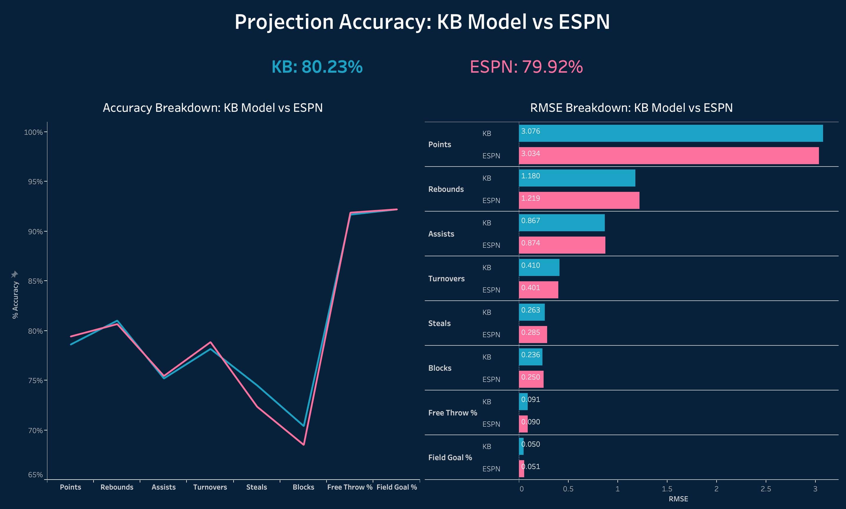
My Model vs ESPN’s Projections below:
Step 1: Webscrapped and wrangled 15+ years of NBA team and player data from basketball-reference.com and espn.com.
- Performed with BeautifulSoup and urlib libraries.
- Looped through the url with the year as a variable
- Parsed through the html to find the proper table
- Appended rows and colums to lists, then converted to numpy array and subsequently a dataframe
- Cleansed the data and added the folllowing variables:
- Position (binary dummy variables)
- Traded? (Different team from last year)
- Starter or Bench Player (40 Game threshold)
- Years Pro
- Stats from 1, 2, and 3 years prior for applicable players
- For college players - Strength of Schedule
Webscraper code:
import requests
from urllib.request import urlopen
from bs4 import BeautifulSoup
import numpy
import pandas as pd

year_to_loop = ['2004','2005','2006','2007','2008','2009','2010','2011','2012','2013','2014','2015','2016','2017','2018','2019']
years = []
players_stats_list_agg = []

#Loop through 15 years
for year in year_to_loop:
    url = 'https://www.basketball-reference.com/leagues/NBA_'+year+'_per_game.html'
    headers= {'User-Agent': 'Mozilla/5.0'}
    response = requests.get(url, headers = headers)
    soup = BeautifulSoup(response.content, 'html.parser')
    stat_table = soup.find_all('table', class_ = 'stats_table')
    stat_table = stat_table[0]

    #append players and stats into players_stats_list
    players_stats_list = []
    for row in stat_table.find_all('tr'):
        for cell in row.find_all('td'):
            players_stats_list_agg.append(cell.text)
            players_stats_list.append(cell.text)

    #append column headers into headers_list
    headers_list = [th.getText() for th in soup.findAll('tr',limit=2)[0].findAll('th')]
    for i in range(int((int(len(players_stats_list)))/(int(len(headers_list)-1)))):
        years.append(year)
- I then converted lists -> arrays -> reshaped and concatenated arrays -> convert to dataframe
The following snippet shows how I added additional variables with an example of starter/benchplayer:
df_stats['Starter'] = (df_stats.GS.astype(int) > 40).astype('int')
Step 2: Built multivariate regression and random forest regresor models for key basketball statistics (points, rebounds, assists, etc) using data pulled in previous setp.
Note: 3 groups of regression and random forest models were built out:
- Players with at least 3 years prior NBA experience
- Players with only 1 or 2 years prior NBA experience
- Rookies
The example below is for group 1 - players with at least 3 years prior NBA experience
Regression Model:
Import libraries and create RMSE Function
import matplotlib.pyplot as plt
import math
import pylab

from scipy import stats
import statsmodels.api as sm

from sklearn.model_selection import train_test_split
from sklearn.linear_model import LinearRegression
from sklearn.metrics import mean_squared_error, r2_score, mean_absolute_error


#function to calculate rmse (root mean squared error)
def rmse(actual, prediction):
    mse = mean_squared_error(actual,prediction)
    rmse = math.sqrt(mse)
    return(rmse)
Build Model and evaluate RMSE:
data_ppg = df_stats[['Age','PTS','PTS_1yp','PTS_2yp','PTS_3yp','MP_1yp','MP_2yp','MP_3yp','PG','SG','SF','PF','Center','Traded','Starter','Years_Pro_Now']]
#Build the model: Define input variable and our output variable (x,y)
X_ppg = data_ppg.drop('PTS', axis=1)
Y_ppg = data_ppg[['PTS']]
#split dataset into training and testing portion
x_train_ppg, x_test_ppg, y_train_ppg, y_test_ppg = train_test_split(X_ppg,Y_ppg, test_size = .20, random_state = 1)
#create an instance of our model
rm_ppg = LinearRegression()
#fit the model
rm_ppg.fit(x_train_ppg,y_train_ppg)
y_predict_ppg = rm_ppg.predict(x_test_ppg)
#evaluate model
X2 = sm.add_constant(X_ppg)
#create OLS model
model_ppg = sm.OLS(Y_ppg,X2)
est_ppg = model_ppg.fit()
print(est_ppg.summary())
#check for normality of residuals
sm.qqplot(est_ppg.resid,line='s')
pylab.show()
print("RMSE: {:.4}".format(rmse(y_test_ppg, y_predict_ppg)))
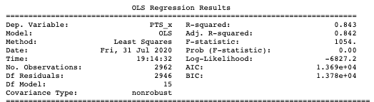
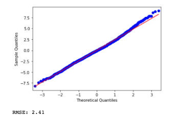
- note: the deviation of the residuals at the top right of the graph indicates heteroscedasticity
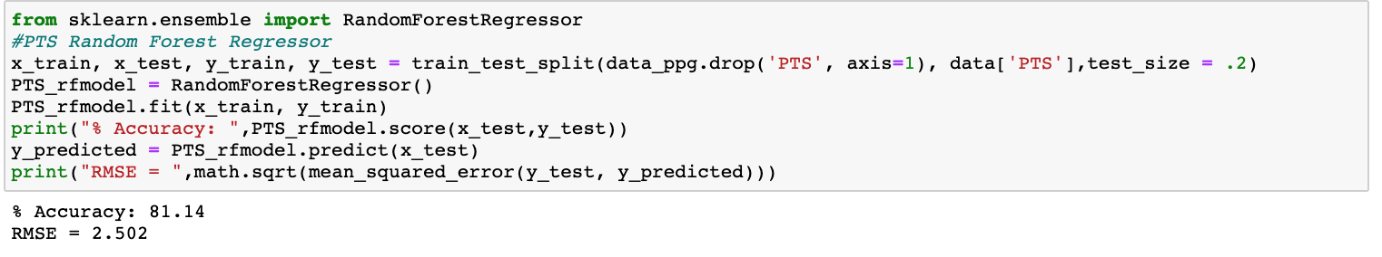
Random Forest Regressor Model:
Step 3: Built a prediction matrix for each basketball statistic and age that calculates league avg percent change (e.g. if the average player’s points per game increases by 8% from when they start the season at age 24 versus age 25, the points prediction for a player turning 25 is 8% more than prior year)
- Building Prediction Matrix:
###Build Matrix:
#Variable to store all player percent change values for each stat
pcnt_change_agg = numpy.arange(15).reshape(1,15)
#loop through each player's career stats and get percent change by year
for player in df_stats['Player'].unique():
    #storing ages
    cnt = df_stats[df_stats.Player ==player].Player.count()
    ages = numpy.asarray(df_stats[df_stats.Player ==player]['Age'].tolist())
    ages = numpy.asarray(ages).reshape(cnt,1)
    #storing percent change for key stats (14 total)
    pcnt_change = df_stats.loc[df_stats.Player ==player][['MP','FGA','FG%','3PA','3P%','eFG%','FTA','FT%','TRB','AST','STL','BLK','TOV','PTS']].replace('','0',regex=True).astype(float).pct_change()
    pcnt_change_array = numpy.asarray(pcnt_change)
    #concatenate ages and pcnt change, then add to aggregate list
    pcnt_change_array = numpy.concatenate([ages,pcnt_change_array], axis=1)
    pcnt_change_agg = numpy.concatenate((pcnt_change_array,pcnt_change_agg), axis=0)
#add column headers to matrix
columns = ['Age','MP','FGA','FG%','3PA','3P%','eFG%','FTA','FT%','TRB','AST','STL','BLK','TOV','PTS']
columns_array = numpy.asarray(columns).reshape(1,15)
pcnt_change_agg = numpy.concatenate([columns_array,pcnt_change_agg], axis=0)
Then:
###convert to dataframe
df_pc_matrix = pd.DataFrame(pcnt_change_agg)
df_pc_matrix.columns = df_pc_matrix.iloc[0]
df_pc_matrix = df_pc_matrix[1:]
df_pc_matrix = df_pc_matrix.astype(float)
#Remove values where pcnt change could not be calculated (e.g a player's rookie year)
df_pc_matrix= df_pc_matrix.replace([numpy.inf, -numpy.inf], numpy.nan)
df_pc_matrix = df_pc_matrix.dropna()
###Create Matrix
df_matrix = pd.DataFrame()
#loop through stat columns and get avgerage pcnt change for each age
for i in columns[1:15]:
    df_matrix[i] = df_pc_matrix.groupby('Age')[i].mean()
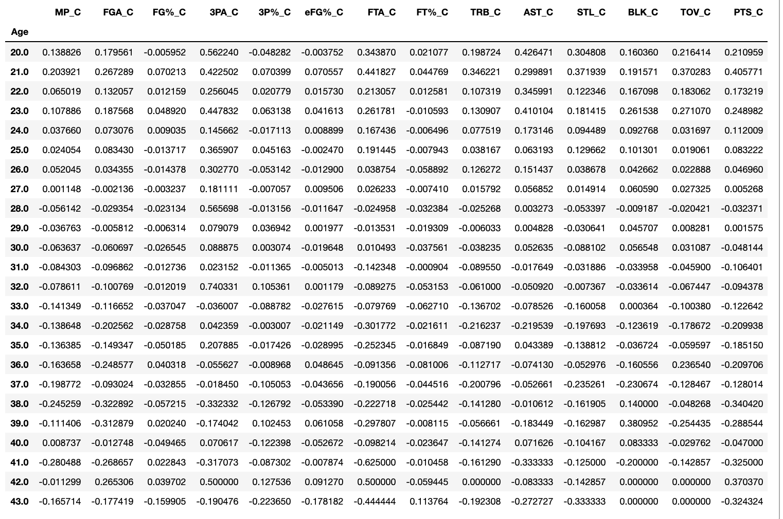
Percent Change by Age Matrix:
- An intersting note is that statistically speaking players on average peak around 27
I then applied the matrix and determined the RMSE:
##Avg Percent Change Matrix Predictions
df_matrix_predict = df_stats[['Player', 'PTS','PTS_1yp', 'Age']].copy()
df_matrix_predict['Age+1'] = df_matrix_predict['Age'].astype(float)+1
df_matrix_predict = pd.merge(df_matrix_predict, df_matrix['PTS_C'], how='inner', left_on=['Age+1'], right_on = ['Age'])
df_matrix_predict['Predict_Bracket'] = (df_matrix_predict['PTS_y'].replace('','0').astype(float) * df_matrix_predict['PTS_C'].replace('','0').astype(float)) + df_matrix_predict['PTS_y'].replace('','0').astype(float)
RMSE(df_matrix_predict.PTS_x, df_matrix_predict.Predict_Bracket)
RMSE = 2.92
- Higher than regression and random forest, but still performed pretty well
4. Conditionally applied prior year weighted averages based on age.
Weighted averages were only applied to players with at least 3 years prior experience as follows:
- 45% * prior year +
- 30% * 2 years prior +
- 25% * 3 years prior
These percentages were established through light trial and error, but applying some sort of optimizer to find the best combination would be a good idea.
###Weighted Averages START
#Function that inputs the weighted average percentages you wish to test
def weighted_avg(y1,y2,y3):
    players_wa = []
    prediction_wa = []
    actual = []
    for player, PTS in df_stats[['Player','PTS']].itertuples(index=False):
        pts1 = df_stats[df_stats.Player == player]['PTS_1yp'].replace('','0').astype(float).reset_index(drop=True) * y1
        pts2 = df_stats[df_stats.Player == player]['PTS_2yp'].replace('','0').astype(float).reset_index(drop=True) * y2
        pts3 = df_stats[df_stats.Player == player]['PTS_3yp'].replace('','0').astype(float).reset_index(drop=True) * y3
        prediction = pts1[0] + pts2[0] + pts3[0]
        players_wa.append(player)
        prediction_wa.append(prediction)
        actual.append(PTS)
    df_wa = pd.DataFrame()
    df_wa['Player'] = players_wa
    df_wa['prediction_wa'] = prediction_wa
    df_wa['PTS'] = actual
    return(RMSE(df_wa.prediction_wa, df_wa.PTS))
#Testing a few different weighted average percentage combinations
print(weighted_avg(.45,.3,.25))
print(weighted_avg(.6,.3,.1))
print(weighted_avg(.5,.3,.2))
RMSE = 4.95
- Much higher than the other 3 methods but we can still check to see if this helps our predictions
Step 5: For rookies - data was pulled from sports-reference.com and only multivariate regression on college stats was used.
Using the 15 years of NBA player data that we have, I created a dataframe with the minimum year for each player and then rejoined to the original table to get a dataframe with just the rookie year stats of each player. I then removed all rows where the minimum year was 2004, as this was most likely not their rookie year but just the last year we pulled data for.
df_min_year = df_stats.groupby('Player')['Year'].min()
df_min_year = pd.merge(df_min_year, df_stats, how = 'inner', left_on = ['Player','Year'], right_on = ['Player','Year'])
df_min_year = df_min_year.drop(df_min_year[df_min_year.Year == '2004'].index)
I then searched through sports-reference.com for each player and their college stats.
###Rookies Data Pull
rookies_agg = numpy.zeros((0,29), dtype=numpy.dtype('U100'))
rookies_agg = numpy.asarray(rookies_agg).reshape(0,29)
#looping through rookie years and formatting player names for url search
for player in df_min_year.Player.replace(' ','-',regex=True):
    player_search = player.replace('.','')
    url = 'https://www.sports-reference.com/cbb/players/'+player.lower()+'-1.html'
    headers= {'User-Agent': 'Mozilla/5.0'}
    response = requests.get(url, headers = headers)
    #condition to check if url exists (200 = does exist)
    if response.status_code == 200:
        soup = BeautifulSoup(response.content, 'html.parser')
        stat_table = soup.find_all('table', class_ = 'stats_table')
        stat_table = stat_table[0]
        stats = []
        for row in stat_table.find_all('tr'):
            for cell in row.find_all('td'):
                stats.append(cell.text)
        #Taking the last 28 columns, these are the stats for last year of college only
        stats = stats[-28:]
        stats.insert(0,player)
        stats = numpy.asarray(stats[0:29])
        stats = numpy.asarray(stats).reshape(1,29)
        rookies_agg = numpy.concatenate((rookies_agg,stats),0)
        headers_list = [th.getText() for th in soup.findAll('tr',limit=2)[0].findAll('th')]
        headers_list.insert(1,'Player')
headers_list = headers_list[1:30]
headers_list = numpy.asarray(headers_list).reshape(1,29)
player_stats = numpy.concatenate((headers_list, rookies_agg),0)
#convert to dataframe
df_rookies = pd.DataFrame(player_stats)
df_rookies.columns = df_rookies.loc[0]
df_rookies = df_rookies.loc[1:]
#undo url formatting of names
df_rookies.Player = df_rookies.Player.replace('-',' ',regex=True)
#join to minimum year so that dataframe contains both last year of college and nba rookie year stats
rookies = pd.merge(df_min_year, df_rookies, how = 'inner',left_on=['Player'], right_on=['Player'])
After adding a player position variable, the data was now ready to be put into multivariate regeression model.
###Rookies Points Per Game
X_ppg = rookies[['PTS_college','MP_college','G_college','GS_college','FGA_college','3P%_college','SOS','PG','SG','SF','PFoward','Center']].astype(float)
Y_ppg = rookies[['PTS']].astype(float)
x_train_ppg, x_test_ppg, y_train_ppg, y_test_ppg = train_test_split(X_ppg,Y_ppg, test_size = .20, random_state = 1)
rm_ppg_rookies = LinearRegression()
rm_ppg_rookies.fit(x_train_ppg,y_train_ppg)
y_predict_ppg = rm_ppg_rookies.predict(x_test_ppg)
#create OLS model
X2 = sm.add_constant(X_ppg)
model_ppg = sm.OLS(Y_ppg,X2)
est_ppg = model_ppg.fit()
print(est_ppg.summary())
sm.qqplot(est_ppg.resid,line='s')
pylab.show()
mean_residuals = sum(est_ppg.resid) / len(est_ppg.resid)
print("RMSE: {:.4}".format(rmse(y_test_ppg, y_predict_ppg)))
RMSE: 3.42
6. Determined which of the 4 methods (regression, random forest, avg % change, and prior year weighted avgs) is most accurate by looking at RMSE and use it for the specific statistic in question for 2020 player predictions.
In our examples above when looking at points per game, we obtained the following RMSEs for our 4 individual methods:
- Regression : 2.41
- Random Forest : 2.50
- % Change Matrix : 2.92
- Weighted Avg : 4.95
I then wanted to check how these methods performed when combined, so I averaged the prediction values for the various methods and determined an RMSE for all 15 combinations.
- Note: the RMSEs are different from the ones listed above because they were run on a different dataset so that none of the models had the advantage of being tested on training data
Results Ranked:
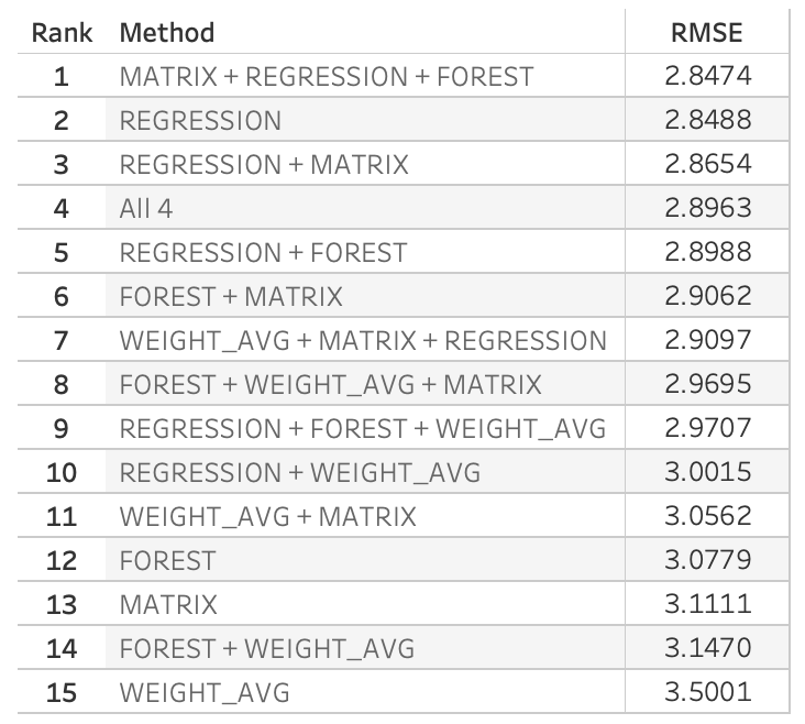
For points, the Matrix + Regression + Forest performed best but only by a slim margin. In general, most methods performed well without significant differences in RMSE.
After creating the new dataset I merged all prediction values from the 4 methods into 1 dataframe:
df_all = pd.DataFrame()
df_all = pd.merge(df_RM[['Player','Year','RM_Predict']],df_RF[['Player','RF_Predict','Year']],how='inner',left_on=['Player','Year'],right_on=['Player','Year'])
df_all = pd.merge(df_all,df_631[['Player','Predict_631','Year']],how='inner',left_on=['Player','Year'],right_on=['Player','Year'])
df_all = pd.merge(df_all,df_bracket[['Player','Predict_Bracket','Year','PTS_x']],how='inner',left_on=['Player','Year'],right_on=['Player','Year'])
df_all.rename(columns={'RM_Predict': 'REGRESSION', 'RF_Predict':'FOREST','Predict_631':'WEIGHT_AVG','Predict_Bracket':'MATRIX','PTS_x': 'ACTUAL'},inplace=True)
I then looped through to create the 15 combinations and tested each method vs the actual:
#list columns so it's easy to copy paste them into a list
df_all.columns
cols = ['REGRESSION', 'FOREST', 'WEIGHT_AVG', 'MATRIX', 'REGRESSION + FOREST', 'REGRESSION + WEIGHT_AVG',
       'REGRESSION + MATRIX', 'FOREST + WEIGHT_AVG', 'FOREST + MATRIX','WEIGHT_AVG + MATRIX',
       'REGRESSION + FOREST + WEIGHT_AVG', 'FOREST + WEIGHT_AVG + MATRIX', 'WEIGHT_AVG + MATRIX + REGRESSION',
       'MATRIX + REGRESSION + FOREST', 'All 4']
methods = []
RMSEs = []
for col in cols:
    methods.append(col)
    RMSEs.append(RMSE(df_all[col], df_all.ACTUAL))
df_RMSE = pd.DataFrame()
df_RMSE['Method'] = methods
df_RMSE['RMSE'] = RMSEs
df_RMSE = df_RMSE.sort_values(by=['RMSE'])
df_RMSE = df_RMSE.reset_index(drop=True)
Step 7: Pulled ESPN’s 2020 season projections from web and merged into a dataframe with my predictions and actual values.
I wanted to compare my model’s performance vs other projections so I searched the internet for 2019-2020 pre-season stat projections. As these would’ve been made in September and we’re currently in July, the only free website I could find with pre-season projections still available was ESPN. The projections were split up into 10 pages on the website, but the url didn’t change when switching pages so I couldn’t figure out a way to webscrape the website.
- I copy pasted the projections from the 10 pages into an excel -> imported into Jupyter Notebook -> formatted the data
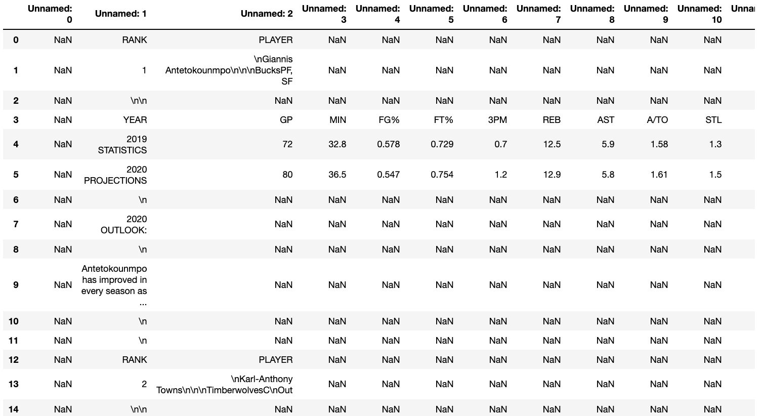
Initial DataFrame:
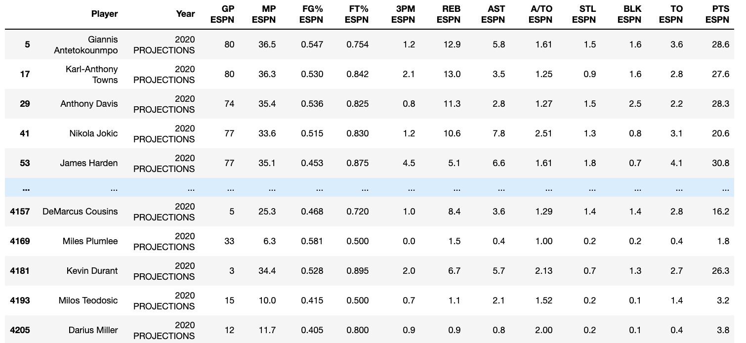
Formatted DataFrame:
Steps to format DataFrame:
###ESPN Projections
data = pd.read_csv('espn bball 2020 projections.csv')

#if string contains \n, then the value in index 4 rows down (+4), 2 columns back (-2) = that same value
for index, i in data[["Unnamed: 2"]].itertuples(index=True):
    if '\n' in str(i):
        data.loc[int(index+4),"Unnamed: 0"] = i
#name columns
columns = ['Player','Year','GP ESPN','MP ESPN','FG% ESPN','FT% ESPN','3PM ESPN','REB ESPN','AST ESPN','A/TO ESPN','STL ESPN','BLK ESPN','TO ESPN','PTS ESPN']
df_columns = pd.DataFrame(columns)
i=0
for col in data.columns:
    data.rename(columns={col:df_columns[0][i]},inplace=True)
    i+=1
espn_proj = data[(data["Year"]=='2020 PROJECTIONS') & (data['MP ESPN'] != '--')]
#Then remove first 2 characters
#then remove everthing starting at \
espn_proj.Player = espn_proj.Player.str[1:]
espn_proj.Player = espn_proj.Player.str.split('\n').str[0]
Frome here, I just merged the this dataframe with my dataframe containing my projections and the actual values.
Step 8: Loaded data into Tableau and calculated % Accuracy as well as RMSE, and performed visual analysis
Projected vs Actual graph, filterable by player and adjustable by specified stat:
Projections vs Actual Player Detail: